Steps 1-6
Load the R packages we will use.
- Read the data in the files,
drug_cos.csv,health_cos.csvin to R and assign to the variablesdrug_cosandhealth_cos, respectively
drug_cos <- read_csv("https://estanny.com/static/week6/drug_cos.csv")
health_cos <- read_csv("https://estanny.com/static/week6/health_cos.csv")
- Use glimpse to get a glimpse of the data
drug_cos %>% glimpse()
Rows: 104
Columns: 9
$ ticker       <chr> "ZTS", "ZTS", "ZTS", "ZTS", "ZTS", "ZTS", "ZTS"~
$ name         <chr> "Zoetis Inc", "Zoetis Inc", "Zoetis Inc", "Zoet~
$ location     <chr> "New Jersey; U.S.A", "New Jersey; U.S.A", "New ~
$ ebitdamargin <dbl> 0.149, 0.217, 0.222, 0.238, 0.182, 0.335, 0.366~
$ grossmargin  <dbl> 0.610, 0.640, 0.634, 0.641, 0.635, 0.659, 0.666~
$ netmargin    <dbl> 0.058, 0.101, 0.111, 0.122, 0.071, 0.168, 0.163~
$ ros          <dbl> 0.101, 0.171, 0.176, 0.195, 0.140, 0.286, 0.321~
$ roe          <dbl> 0.069, 0.113, 0.612, 0.465, 0.285, 0.587, 0.488~
$ year         <dbl> 2011, 2012, 2013, 2014, 2015, 2016, 2017, 2018,~
health_cos %>% glimpse()
Rows: 464
Columns: 11
$ ticker      <chr> "ZTS", "ZTS", "ZTS", "ZTS", "ZTS", "ZTS", "ZTS",~
$ name        <chr> "Zoetis Inc", "Zoetis Inc", "Zoetis Inc", "Zoeti~
$ revenue     <dbl> 4233000000, 4336000000, 4561000000, 4785000000, ~
$ gp          <dbl> 2581000000, 2773000000, 2892000000, 3068000000, ~
$ rnd         <dbl> 427000000, 409000000, 399000000, 396000000, 3640~
$ netincome   <dbl> 245000000, 436000000, 504000000, 583000000, 3390~
$ assets      <dbl> 5711000000, 6262000000, 6558000000, 6588000000, ~
$ liabilities <dbl> 1975000000, 2221000000, 5596000000, 5251000000, ~
$ marketcap   <dbl> NA, NA, 16345223371, 21572007994, 23860348635, 2~
$ year        <dbl> 2011, 2012, 2013, 2014, 2015, 2016, 2017, 2018, ~
$ industry <chr> "Drug Manufacturers - Specialty & Generic", "Dru~- Which variables are the same in both data sets
names_drug <- drug_cos %>% names()
names_health <- health_cos %>% names()
intersect(names_drug, names_health)
[1] "ticker" "name" "year" - Select subset of variables to work with
For
drug_cosselect (in this order):ticker,year.grossmarginExtract observations for 2018
assign output to
drug_subset
For
health_cosselect in order:ticker,year,revenue,gp,industryextract observations for 2018
Assign output to
health_subset
- Keep all the rows and columns
drug_subsetjoin with columns inhealth_subset
drug_subset %>% left_join(health_subset)
# A tibble: 13 x 6
   ticker  year grossmargin   revenue        gp industry
   <chr>  <dbl>       <dbl>     <dbl>     <dbl> <chr>
 1 ZTS     2018       0.672   5.82e 9   3.91e 9 Drug Manufacturers - ~
 2 PRGO    2018       0.387   4.73e 9   1.83e 9 Drug Manufacturers - ~
 3 PFE     2018       0.79    5.36e10   4.24e10 Drug Manufacturers - ~
 4 MYL     2018       0.35    1.14e10   4.00e 9 Drug Manufacturers - ~
 5 MRK     2018       0.681   4.23e10   2.88e10 Drug Manufacturers - ~
 6 LLY     2018       0.738   2.46e10   1.81e10 Drug Manufacturers - ~
 7 JNJ     2018       0.668   8.16e10   5.45e10 Drug Manufacturers - ~
 8 GILD    2018       0.781   2.21e10   1.73e10 Drug Manufacturers - ~
 9 BMY     2018       0.71    2.26e10   1.60e10 Drug Manufacturers - ~
10 BIIB    2018       0.865   1.35e10   1.16e10 Drug Manufacturers - ~
11 AMGN    2018       0.827   2.37e10   1.96e10 Drug Manufacturers - ~
12 AGN     2018       0.861   1.58e10   1.36e10 Drug Manufacturers - ~
13 ABBV    2018       0.764   3.28e10   2.50e10 Drug Manufacturers - ~
Question: join_ticker
. Start with the drug_cos data
. Extract observations for the ticker MRK from drug_cos . Assign output to the variables drug_cos_subset
drug_cos_subset <- drug_cos %>%
  filter(ticker == "MRK")
. Display drug_cos_subset
drug_cos_subset
# A tibble: 8 x 9
  ticker name  location ebitdamargin grossmargin netmargin   ros   roe
  <chr>  <chr> <chr>           <dbl>       <dbl>     <dbl> <dbl> <dbl>
1 MRK    Merc~ New Jer~        0.305       0.649     0.131 0.15  0.114
2 MRK    Merc~ New Jer~        0.33        0.652     0.13  0.182 0.113
3 MRK    Merc~ New Jer~        0.282       0.615     0.1   0.123 0.089
4 MRK    Merc~ New Jer~        0.567       0.603     0.282 0.409 0.248
5 MRK    Merc~ New Jer~        0.298       0.622     0.112 0.136 0.096
6 MRK    Merc~ New Jer~        0.254       0.648     0.098 0.117 0.092
7 MRK    Merc~ New Jer~        0.278       0.678     0.06  0.162 0.063
8 MRK    Merc~ New Jer~        0.313       0.681     0.147 0.206 0.199
# ... with 1 more variable: year <dbl>
. Use left_join to combine rows and columns of drug_cos_subset with the columns of health_cos
. Assign The output to combo_df
combo_df <- drug_cos_subset %>%
  left_join(health_cos)
. Display combo_df
combo_df
# A tibble: 8 x 17
  ticker name  location ebitdamargin grossmargin netmargin   ros   roe
  <chr>  <chr> <chr>           <dbl>       <dbl>     <dbl> <dbl> <dbl>
1 MRK    Merc~ New Jer~        0.305       0.649     0.131 0.15  0.114
2 MRK    Merc~ New Jer~        0.33        0.652     0.13  0.182 0.113
3 MRK    Merc~ New Jer~        0.282       0.615     0.1   0.123 0.089
4 MRK    Merc~ New Jer~        0.567       0.603     0.282 0.409 0.248
5 MRK    Merc~ New Jer~        0.298       0.622     0.112 0.136 0.096
6 MRK    Merc~ New Jer~        0.254       0.648     0.098 0.117 0.092
7 MRK    Merc~ New Jer~        0.278       0.678     0.06  0.162 0.063
8 MRK    Merc~ New Jer~        0.313       0.681     0.147 0.206 0.199
# ... with 9 more variables: year <dbl>, revenue <dbl>, gp <dbl>,
#   rnd <dbl>, netincome <dbl>, assets <dbl>, liabilities <dbl>,
# marketcap <dbl>, industry <chr>- Note: the variables
ticker,name,locationandindustryare the same for all the observations
. Assign the company name to co_name
co_name <- combo_df %>%
  distinct(name) %>%
  pull()
. Assign the company location to co_location
co_location <- combo_df %>%
  distinct(location) %>%
  pull()
. Assign the industry to co_industry group
co_industry <- combo_df %>%
  distinct(industry) %>%
  pull()
The company Merck & Co Inc is located in New Jersey; U.S.A and is a member of the Drug Manufacturers - General industry group.
. Start with combo_df
. Select variables (in this order): year, grossmargin, netmargin, revenue, gp, netincome
. Assign the output to combo_df_subset
combo_df_subset <- combo_df %>%
  select(year, grossmargin, netmargin, revenue, gp, netincome)
. Display combo_df_subset
combo_df_subset
# A tibble: 8 x 6
   year grossmargin netmargin     revenue          gp   netincome
  <dbl>       <dbl>     <dbl>       <dbl>       <dbl>       <dbl>
1  2011       0.649     0.131 48047000000 31176000000  6272000000
2  2012       0.652     0.13  47267000000 30821000000  6168000000
3  2013       0.615     0.1   44033000000 27079000000  4404000000
4  2014       0.603     0.282 42237000000 25469000000 11920000000
5  2015       0.622     0.112 39498000000 24564000000  4442000000
6  2016       0.648     0.098 39807000000 25777000000  3920000000
7  2017       0.678     0.06  40122000000 27210000000  2394000000
8  2018       0.681     0.147 42294000000 28785000000  6220000000
. Create the variables grossmargin_check to compare with the variables grossmargin. They should be equal - grossmargin_check = gp / revenue
. Create the variable close_enough to check the absolute value of the difference between grossmargin_check and grossmargin is less than 0.00
combo_df_subset %>%
  mutate(grossmargin_check = gp / revenue,
  close_enough = abs(grossmargin_check - grossmargin) < 0.001)
# A tibble: 8 x 8
   year grossmargin netmargin     revenue          gp   netincome
  <dbl>       <dbl>     <dbl>       <dbl>       <dbl>       <dbl>
1  2011       0.649     0.131 48047000000 31176000000  6272000000
2  2012       0.652     0.13  47267000000 30821000000  6168000000
3  2013       0.615     0.1   44033000000 27079000000  4404000000
4  2014       0.603     0.282 42237000000 25469000000 11920000000
5  2015       0.622     0.112 39498000000 24564000000  4442000000
6  2016       0.648     0.098 39807000000 25777000000  3920000000
7  2017       0.678     0.06  40122000000 27210000000  2394000000
8  2018       0.681     0.147 42294000000 28785000000  6220000000
# ... with 2 more variables: grossmargin_check <dbl>,
#   close_enough <lgl>
. Create the variable netmargin_check to compare with the variable netmargin. They should be equal.
. Create the variable close_enough to check that the absolute value of the differences between netmargin_check and netmargin is less than 0.001
combo_df_subset %>%
  mutate(netmargin_check = netincome / revenue,
  close_enough = abs(netmargin_check -  netmargin) <0.001)
# A tibble: 8 x 8
   year grossmargin netmargin     revenue          gp   netincome
  <dbl>       <dbl>     <dbl>       <dbl>       <dbl>       <dbl>
1  2011       0.649     0.131 48047000000 31176000000  6272000000
2  2012       0.652     0.13  47267000000 30821000000  6168000000
3  2013       0.615     0.1   44033000000 27079000000  4404000000
4  2014       0.603     0.282 42237000000 25469000000 11920000000
5  2015       0.622     0.112 39498000000 24564000000  4442000000
6  2016       0.648     0.098 39807000000 25777000000  3920000000
7  2017       0.678     0.06  40122000000 27210000000  2394000000
8  2018       0.681     0.147 42294000000 28785000000  6220000000
# ... with 2 more variables: netmargin_check <dbl>,
#   close_enough <lgl>
Question summarize_industry
- for each industry calculate
- mean_netmargin_percent = mean(netincome / revenue) * 100
- median_netmargin_percent = median(netincome / revenue) * 100
- min_netmargin_percent = min(netincome / revenue) * 100
- max_netmargin_percent = max(netincome / revenue) * 100
health_cos %>%
  group_by(industry) %>%
  summarize(mean_netmargin_percent = mean(netincome / revenue) * 100,
            median_netmargin_percent = median(netincome / revenue) * 100,
            min_netmargin_percent = min(netincome / revenue) * 100,
            max_netmargin_percent = max(netincome / revenue) * 100)
# A tibble: 9 x 5
  industry       mean_netmargin_pe~ median_netmargin~ min_netmargin_p~
  <chr>                       <dbl>             <dbl>            <dbl>
1 Biotechnology               -4.66              7.62         -197.
2 Diagnostics &~              13.1              12.3             0.399
3 Drug Manufact~              19.4              19.5           -34.9
4 Drug Manufact~               5.88              9.01          -76.0
5 Healthcare Pl~               3.28              3.37           -0.305
6 Medical Care ~               6.10              6.46            1.40
7 Medical Devic~              12.4              14.3           -56.1
8 Medical Distr~               1.70              1.03           -0.102
9 Medical Instr~              12.3              14.0           -47.1
# ... with 1 more variable: max_netmargin_percent <dbl>
Question: inline_ticker
- Extract observations for the ticker BMY from
health_cosand assign to the variablehealth_cos_subset
health_cos_subset <- health_cos %>%
  filter(ticker == "BMY")
- Display
health_cos_subset
health_cos_subset
# A tibble: 8 x 11
  ticker name     revenue      gp    rnd netincome  assets liabilities
  <chr>  <chr>      <dbl>   <dbl>  <dbl>     <dbl>   <dbl>       <dbl>
1 BMY    Bristo~  2.12e10 1.56e10 3.84e9    3.71e9 3.30e10 17103000000
2 BMY    Bristo~  1.76e10 1.30e10 3.90e9    1.96e9 3.59e10 22259000000
3 BMY    Bristo~  1.64e10 1.18e10 3.73e9    2.56e9 3.86e10 23356000000
4 BMY    Bristo~  1.59e10 1.19e10 4.53e9    2.00e9 3.37e10 18766000000
5 BMY    Bristo~  1.66e10 1.27e10 5.92e9    1.56e9 3.17e10 17324000000
6 BMY    Bristo~  1.94e10 1.45e10 5.01e9    4.46e9 3.37e10 17360000000
7 BMY    Bristo~  2.08e10 1.47e10 6.48e9    1.01e9 3.36e10 21704000000
8 BMY    Bristo~  2.26e10 1.60e10 6.34e9    4.92e9 3.50e10 20859000000
# ... with 3 more variables: marketcap <dbl>, year <dbl>,
#   industry <chr>
In the console, type
?distinct. Go to the help pane to see wahtdisticntdoesIne the console, type
?pull. Go to the help pane to see what it does.Run the code below
health_cos_subset %>%
  distinct(name) %>%
  pull(name)
[1] "Bristol Myers Squibb Co"- Assign the output to
co_name
co_name <- health_cos_subset %>%
  distinct(name) %>%
  pull(name)
- The name of the company ticker BMY is Bristol Myers Squibb Co
In following chunk
- Assign the comapnys industry group to the variable
co_industry
co_industry <- health_cos_subset %>%
  distinct(industry) %>%
  pull()
The company Bristol Myers Squibb Co is a member of Drug Manufacturers - General
Steps 7-11
- Prepare the data for the plots
- starts with health_cos THEN
- group_by industry THEN
- calculate the median research and development expenditure by industry
- assign the output to
df
- Use
glimpseto glimpse the data for the plots
df %>% glimpse()
Rows: 9
Columns: 2
$ industry    <chr> "Biotechnology", "Diagnostics & Research", "Drug~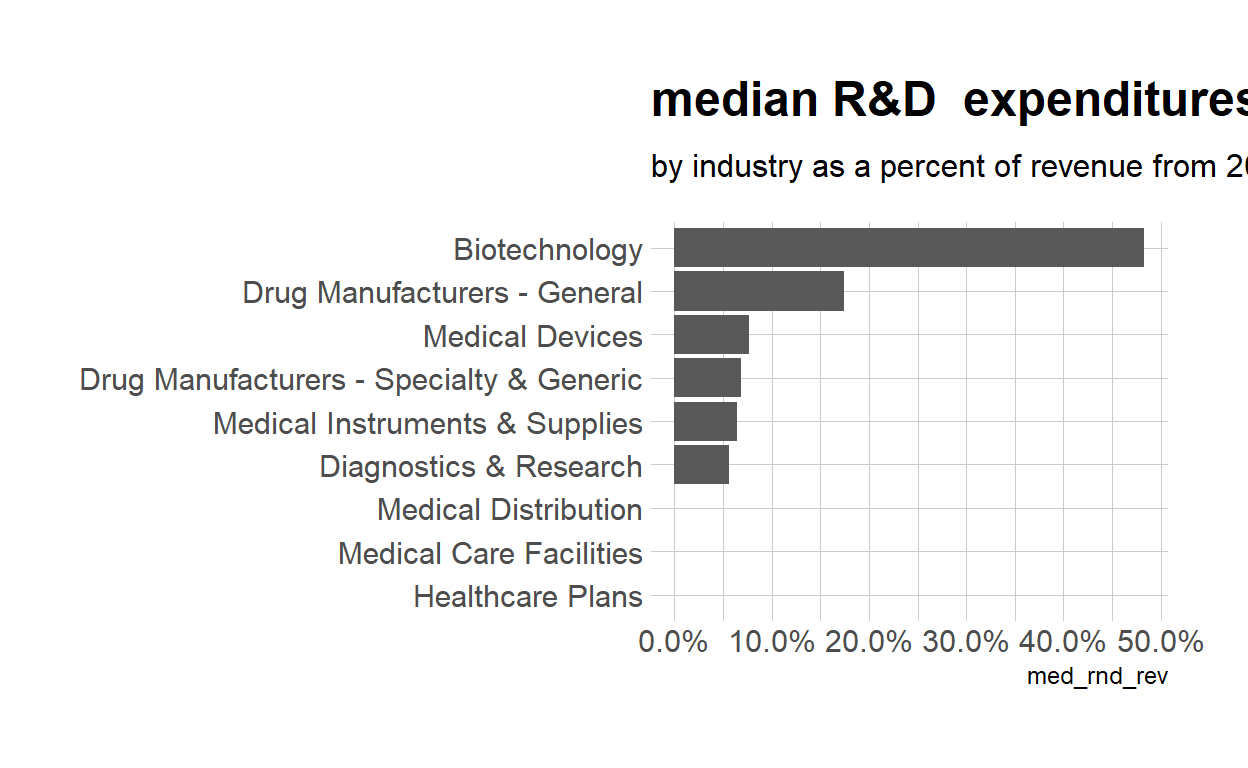
$ med_rnd_rev <dbl> 0.48317287, 0.05620271, 0.17451442, 0.06851879, ~- Create a static bar chart
- use
ggplotto initailize the chart - data is
df - the variable
industryis mapped to the x-axis -reorder it based the value ofmed_rnd_rev - the variable
med_rnd_revis mapped on the y axis - add a bar chart using
geom_col - use
scale_y_contnuousto label the y-axis with percent - use
cord_flip()to flip the coordiantes - use
labsto add title, subtitle and remove x and y axes - use
theme_ipsum()from the hrbrthemes package to improve the theme
ggplot(data = df, mapping = aes(
  x = reorder(industry, med_rnd_rev ),
  y = med_rnd_rev
)) +
  geom_col() +
  scale_y_continuous(labels = scales::percent) +
  coord_flip() +
  labs(
    title = "median R&D  expenditures",
    subtitle = "by industry as a percent of revenue from 2011 to 2018",
    x = NULL, Y = NULL) +
  theme_ipsum()
- Save the last plot to preview.png and add the yaml chunk at the top
ggsave(filename = "preview.png", path = here::here("_posts", "2021-03-16-joining-data"))
Create an interactive bar chart using the package echarts4r -start with the data df -use arrange to reorder med_rnd_rev -use e_charts to initialize a chart -the variable industry is mapped to the x-axis -add a bar chart using e_bar with the values of med_rnd_rev -use e_flip_coords() to flip the coordinates -use e_title to add the title and the subtitle -use e_legend to remove the legends -use e_x_axis to change format of labels on x-axis to percent -use e_y_axis to remove labels on y-axis- -use e_theme to change the theme. Find more themes here
df %>%
  arrange(med_rnd_rev) %>%
  e_charts(
    x = industry
  ) %>%
  e_bar(
    serie = med_rnd_rev,
    name = "median"
  ) %>%
  e_flip_coords() %>%
  e_tooltip() %>%
  e_title(
    text = "median industry R&D expenditures",
    subtext = "by industry as a percent of revenue from 2011 to 2018",
    left = "center") %>%
  e_legend(FALSE) %>%
  e_x_axis(
    formatter = e_axis_formatter("percent", digits = 0)
  ) %>%
  e_y_axis(
    show = FALSE
  ) %>%
  e_theme("infographic")